Understanding Bézier Curves

Bézier curves are everywhere. In your CSS animation timing function, in graphic editors, in typography, in car design and much, much more. If you want to model a smooth curve, chances are you’ll probably end up using a Bézier curve.

I think these curves are a perfect example of applied mathematics and its influence on our day-to-day lives as developers. Even though we might not want to understand every single mathematical aspect of what’s underneath our cosy abstractions (I certainly don’t) , I think it’s good to sometimes peek under the hood and see what things are actually made of.

This is my goal with this article. After it, you’ll have a mathematical and intuitive understanding of what exactly is a Bézier curve, why do we use them and how they work.

What is a Bézier curve?

Bézier curves are parametric curves that are defined by a set of control points. These points’ position’s in relation to one another defined the shape of the curve.

If you’ve ever used a graphic editing software like Adobe Illustrator or Figma, you’ve already seen these control points in action. Notice in the gif below how as the points move, the curve’s shape changes accordingly.

You can also use as many control points as you like. The more of them you have, the greater the control that you have over the final shape of your curve. As an example, the cubic-bezier function in CSS uses a curve with 4 points (hence cubic) that describe the evolution of your animation.

What’s going on?

That’s great and all, but how do get a smooth curve from just positioning a bunch of points around?

The answer to that is in the mathematical basis for Bézier curves, the Bernstein polynomials. A Bernstein polynomial $B_n(x)$ of degree $n$ is defined as a sum of Bernstein basis polynomials $b_{v,n}(x)$, each multiplied by a Bernstein coefficient $\beta_v$. Here’s the formula for the Bernstein polynomial:

And for the Bernstein basis polynomial:

Don’t get hung up on these formulas, there’s only a few key things you need to take from them.

First, what is their purpose? Well, to make a long story short, Bernstein polynomials are mainly used as a way to approximate real continuous functions within a closed interval (see Stone-Weierstrass theorem for more details). In other words, by using these polynomials, we can approximate practically any function (model any curve) that we want to. This is really useful, as polynomials are generally a lot simpler to evaluate and manipulate that other types of functions.

Second, how does this approximation actually work? If you take a closer look at the formula for $B_n(x)$, you won’t see any immediate hints on how is it that it can approximate a real function $f$. Actually, it takes a slight modification in the formula to make that possible:

Notice how now one of the parameters received is a function $f$, and also that we substitute the Bernstein coefficient $\beta_v$ with $f(\frac{v}{n})$. This makes sense, as we need to make the $B_n(x)$ dependant on $f$ (or its values) in some way so that it can approximate it. Since the basis polynomials $b_{v,n}$ depends only on $x$ and $n$, the coefficients $\beta_v$ take on the role of actually approximating the target function.

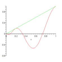
It can be proven that $B_n(f)$ equals $f$ more and more for increasing values of $n$. In other words, $\lim_{n \to \infty}B_n(f) = f$.

But how does all of this relate to Bézier curves? Well, one of the ways Bézier curves are defined is via what’s called their explicit definition, depicted below, with $P_i$ being the ith control point of the curve:

Notice any similarities? This is exactly the formula for a Bernstein polynomial, but with $P_i$ taking the place of the Bernstein coefficient! Therefore, we can say that a Bézier curve is actually a Bernstein polynomial, but with the control points taking the place of its Bernstein coefficients!

There’s still another way of looking at Bézier curves, which I think is more powerful and intuitive, which is what we’ll explore now.

A different approach

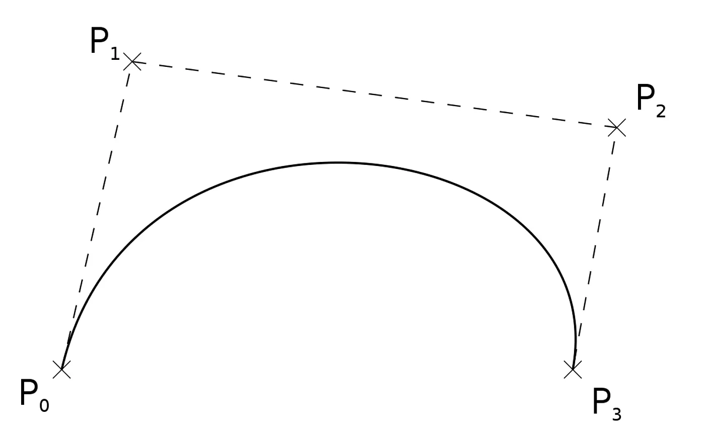
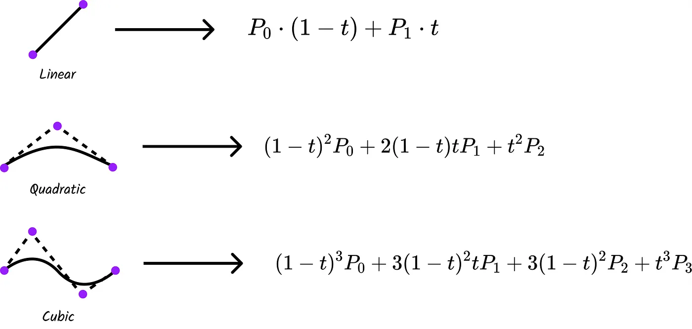
There are a few famous form of Bézier curves, which are based on its amount of control points (its degree). They are the linear, quadratic and cubic Bézier curves. When studying this topic, you’ll probably encounter their formulas, which you can obtain by applying the explicit definition we showed previously:

Again, don’t get hung up on these formulas. There’s only one key thing you need to take from them.

Pay close attention to the formula of the linear Bézier curve. Notice how we have $(1 - t)$ and $t$ times something. Without context, there’s nothing special about it, it’s just basic linear interpolation. But look what happens when we move things around a bit in the quadratic formula:

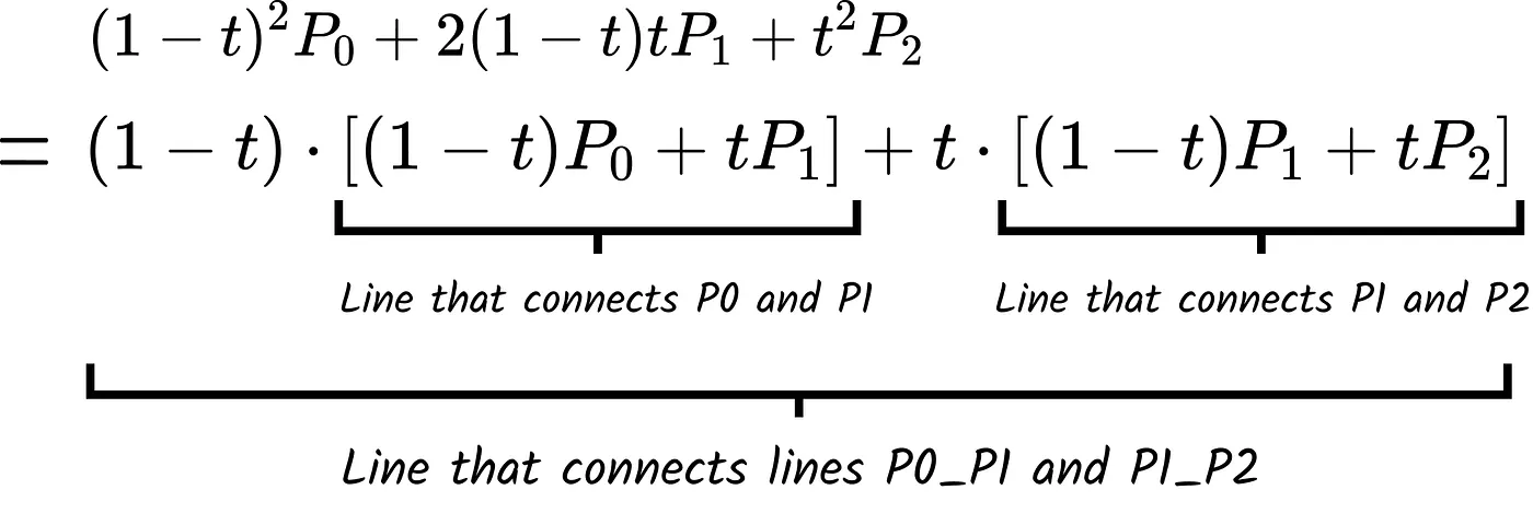
The pattern $(1 - t)$ and $t$ times something (linear interpolation) repeats itself. We’re representing the quadratic curve as a linear interpolation of two other linear interpolations (go back to the previous image with different types of Bézier curves and notice the lines connecting the control points). This hints at a new way to define Bézier curves, in terms of themselves, i.e., recursively:

Thus, a Bézier curve with a set of control points $P_0, P_1, \dots, P_n$ can also be defined as a linear interpolation of two lower-degree Bézier curves whose control points are subsets of the original ones.

This also means that we get a new way to evaluate a point in a Bézier curve, different from our original way that stems from the Bernstein polynomials.

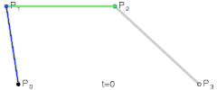
Imagine that we’re trying to calculate the point $t = 0.5$ in a quadratic Bézier curve $B_{P_0, P_1, P_2}$. We just saw that we can represent this curve as the linear interpolation of two linear Bézier curves $B_{P_0,P_1}$ and $B_{P_1, P_2}$. By plugging $0.5$ in our new recursive formula, we calculate $t=0.5$ in $B_{P_0, P_1}$ and then in $B_{P_1, P_2}$ - which gives us two new points -, to then connect these two intermediate points with another linear interpolation and calculate the final position of $t = 0.5$.

Let me give you a visualization of what’s going on:

For each evaluated point $t$, we actually calculate it first in each of the lower degree curves, to then connect them and calculate the desired point in the resulting line. This patterns repeats with higher-level curves as well:

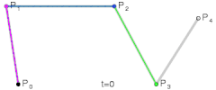
It’s almost as if the hidden lines define the “skeleton” (the boundaries) of the resulting curve. Pretty awesome.

Understanding this is important, as it is the explanation for a special topic that always comes up when studying Bézier curves: De Casteljau’s algorithm.

De Castelijau’s algorithm

This famous algorithm essentially uses the recursive definition to evaluate each point of the curve. It divides the calculation in levels, with the first level having the individual control points, the final level having your desired point, and the middle ones having all the intermediate points we calculate throughout the recursive definition. Let’s see how it works with a cubic curve:

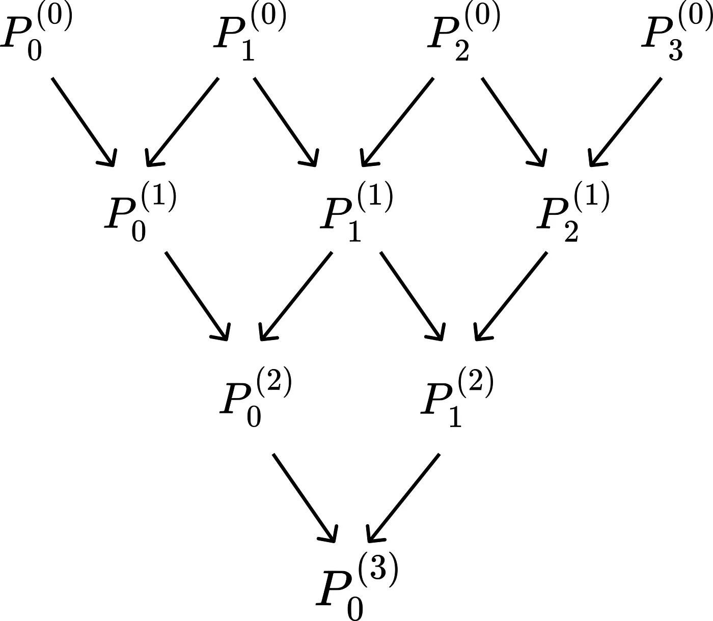
Therefore, given that each point on level 0 is the control point itself, and considering that $P_i^(j)$ represents the ith point at level $j$ (not exponentiation!) , De Casteljau’s algorithm tells us that its value will be:

Always remember that this is essentially using the recursive pattern in the Bézier curves, which are derived from the Bernstein polynomials.

Why Bézier curves?

Given everything we’ve said about Bézier curves, what’s the big deal with them? Why do we use them so much?

Essentially, they’re a way to build curves that can be scaled indefinitely, meaning that we can make them as detailed as we want them to be. Instead of creating super high degree curves, we can just concatenate smaller degree curves together and get pretty much any curve we want to.

Take the prime example of typography. Bézier curves enable us to create all kinds of different fonts, from simple monospace to beautiful display ones!

A final overview

To sum up everything we’ve learned in this article:

• Bézier curves are parametric curves that are defined by a set of control ponts
• Their mathematical origins come from the Bernstein polynomials, which are a way to approximate real functions.
• Bézier curves are Bernstein polynomials with the control points taking the place of Bernstein coefficients.
• Bézier curves are recursive, and each curve $B_{P_0, \dots, P_n}$ points can be represented as linear interpolation of the Bézier curves $B_{P_0, \dots, P_{n-1}}$ $B_{P_1, \dots, P_{n}}$.
• De Casteljau’s algorithm essentially uses this recursive relation to calculate an arbitrary point of a Bézier curve.
• Bézier curves are really useful because they can be scaled indefinitely and allows us to create basically any curve that we want to.