AVL trees: A comprehensive explanation

I’ve always had some difficulty when it came to understanding balanced trees. I don’t know why, but it was never easy for my brain to understand their seemingly arbitrary definitions and how they lead to guaranteed efficiency for the search, insert and delete operations.

After a considerable amount of effort, I’ve reached a place where I feel somewhat comfortable with my understanding of these data structures. So I thought, “why not turn this into a series of blog posts and see if I actually understand what I’m talking about?“.

This article is the first in this series, and it will be about AVL trees. First, I’ll quickly explain the motivation behind balanced tree, then I’ll introduce and comprehensively explain AVL trees and how they work.

An important disclaimer: I assume that you are already familiar with binary search trees.

It’s all about balance

People normally encounter AVL trees as their first type of height balanced trees. But what exactly is a height balanced tree? They are binary trees whose height $h$ is within a constant factor of $\lfloor log_2^{n + 1}\rfloor$, with $n$ being the number of nodes (i.e., $h$ is $\Theta(log_2^{n + 1})$). Since the minimum height for a binary tree is $\lfloor log_2^{n + 1}\rfloor - 1$, this works great.

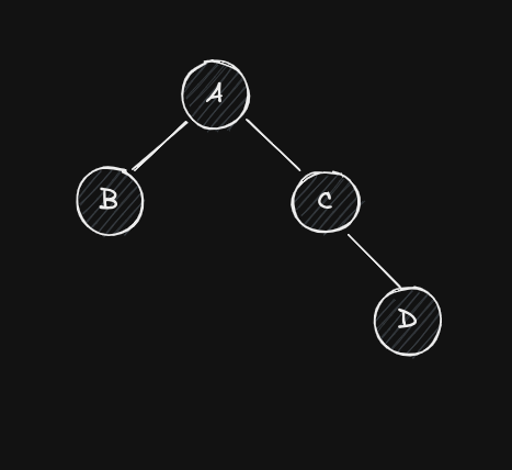
Why is this necessary? Because, by themselves, binary (search) trees don’t guarantee good performance, as they can grow to become too tall and thus compromise the speed of their operations. For example, here are three different binary trees with the same set of values:

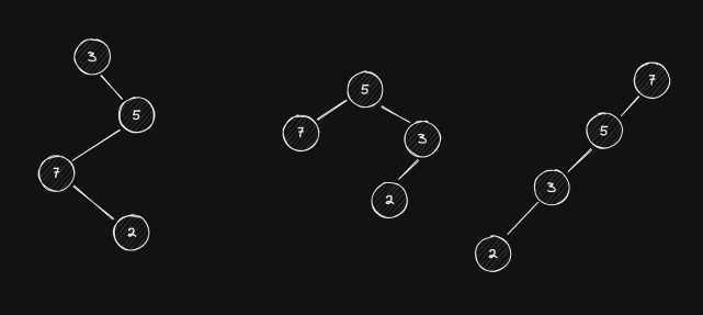
If we were to search for the element 2 in all of them, the amount of comparisons we’d have to make with the middle tree would be less than with the ones at the sides (these actually just degrade into linear searches). This is because of the tree’s height. Thus, it makes sense to create a tree structure that guarantees its height is close to the absolute minimum.

AVL trees

An AVL tree is a binary tree such that, for every node $v$, the difference in height between $v$’s right and left subtree is not greater than one. For any node $v$, its balance factor $BF$ is given by:

Where $H(x)$ is the height of the binary tree with root $x$ and $v_r$ and $v_l$ are $v$’s right and left subtree, respectively. Thus, an AVL tree is a binary tree such that, for every node $v$, $-1 \leq BF(v) \leq 1$.

The following image shows a common way to represent AVL trees. Notice how the node’s balance factor is now represented at the center of the circle, with the node’s label (or value) at its side. Symbols $\cdot$, $+$ and $-$ represent balance factors, 0, +1 and -1, respectively. Any tree that contains a node with balance factor greater than 1 or less than -1 (like $C$ with $BF$ +2) is said to be unbalanced. A node that has balance factor greater than 0 is said to be right-heavy, while a node with balance factor less than 0 is called left-heavy.

AVL trees can become unbalanced after insert/delete operations, as these can change the tree’s height ($C$ could have become unbalanced after the insertion of $H$ or after the removal of its left node). If such a state occurs, then rebalancing is needed. As these operations can’t change the tree’s height by more than 1 unit, balance factors greater than +2 or less than -2 don’t appear. Thus, any unbalanced state requires at least one node with a balance factor of +2 or -2.

Since AVL trees are also binary search trees, their core operations (search/insert/delete) are very similar to regular BST ones. The only differences reside in the insert and delete operations. Since they can change the tree’s height, we need to verify, after performing them, if the tree is still balanced, and if it isn’t, we need to rebalance it.

Rotations

Before diving into specifics, we need to understand rotations, as they are crucial in the process of rebalancing AVL trees.

A rotation is an operation performed on a node $v$ of a binary tree, such that $v$ will “go down” and one of its children will assume its place. If it’s a left rotation, then $v$’s right child takes its place, and if it’s a right rotation, then $v$’s left child take its place.

A rotation changes the structure of a binary tree, but it doesn’t invalidate its order. Meaning, if a tree is a binary search tree before a rotation, it remains so after the rotation. The following image shows the effects of left/right rotations.

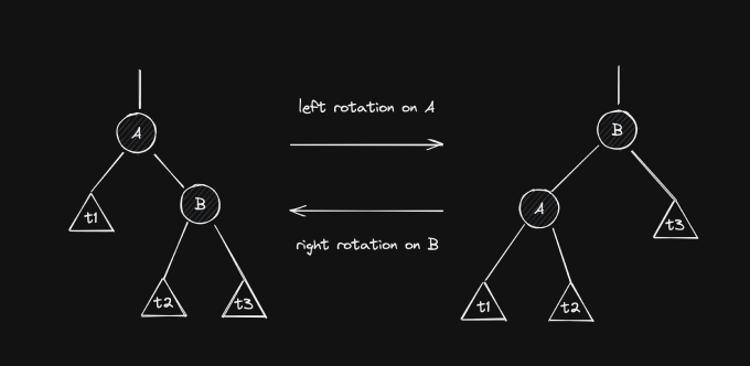
Here, $A$ and $B$ are individual nodes and $t_1$, $t_2$ and $t_3$ are general subtrees, which can be empty.

Let’s take a closer look at the left rotation on $A$. If $A$ is left-rotated, then it becomes $B$’s left child. Therefore, we need to find a new place for $B$’s previous left child, $t_2$. From the initial layout of the tree, we know that $A < t_2 < B$. Thus, if we put it as $A$’s right child, we preserve the order of the entire tree. The right rotation is simply a mirrored version of this case (you’re encouraged to check why it’s also valid).

There are two other important points that we need to take from this diagram. First, notice how $A$ and $B$ can be children of other nodes. It’s perfectly valid (and very common) to perform rotations on subtrees. Lastly, notice how the height of the node that goes down decreases by one and the height of the node that takes its place increases by one. This will be useful when rebalancing AVL trees.

Rebalancing

The only real difference between AVL trees and binary search trees is that, in some cases, the former requires rebalancing after insertion/removal. I say “only” not because I think it’s super simple to understand these cases, but because I think they’re the key to real understanding understanding of AVL trees. If you really get familiar with them, then implementing an AVL tree becomes much simpler.

Let’s start with the case of a tree $T_v$ with root $v$ such that $BF(v) = 2$. For this to occur, one of two things happened:

• $v$’s left subtree became shorter (a node was removed)
• $v$’s right subtree became taller (a node was added)

Since insertion and removal can change a tree’s height by at most 1 unit, we know that, prior to any of these two cases, $v$’s balance factor was +1. This means that the initial layout was something like this:

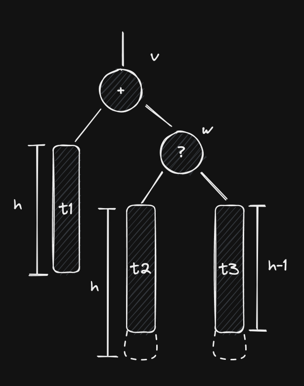
Since $v$ is right-heavy, then it must have at least one node on its right subtree, here named $w$. We can’t say much about $w$ right now, but we’re going to assume that it’s balanced. As a matter of fact, we’re going to assume that both of $v$’s subtrees are balanced. Because of this, and because $v$ is right-heavy, we know that at least one of $w$’s subtrees must have height equal to $h$, while the other may have height $h-1$ or $h$.

Now that we’ve established the initial layout of the tree, we can analyze specific cases where $v$ becomes unbalanced.

Case 1: Insertion in $v$’s right subtree

Our first new assumption is that $v$ became unbalanced after an insertion of a new node $n$ on its right subtree. We know that $n \neq w$, since $w$ was around before the insertion. Thus, $n$ is either in $t_2$ or in $t_3$.

Before diving into these sub-cases, there are still some things that we can deduce. If the insertion of $n$ increased the height of $v$’s right subtree, then it must have done the same to one of $w$’s subtrees. For this to happen while $v$ remains as the unbalanced node that’s closest to the trees, then, prior to the insertion, $w$’s balance factor must have been equal to 0!

The best way to understand this is to imagine what would happen if $w$’s balance factor were equal to -1 or +1. If it was equal to -1 prior to the insertion, only two things could have happened after it:

• $n$ goes into $w$’s left subtree, which increases its height by one, making $w$’s balance factor equal to -2. This contradicts our initial hypothesis that $v$ was the unbalanced node closets to the leaves.
• $n$ goes into $w$’s right subtree, which increases its height by one, making $w$’s balance factor equal to 0. This doesn’t increase $w$’s total height (neither that of the tree), also contradicting our initial assumption that the tree becomes unbalanced after the insertion.

Since both cases result in contradictions, then the initial assumption is deemed impossible. The analysis for if $BF(w) = 1$ is a mirrored version of this one. Thus, prior to the insertion, we know that $BF(w) = 0$. This means that our tree initially looked like this:

Now let’s look at some sub-cases.

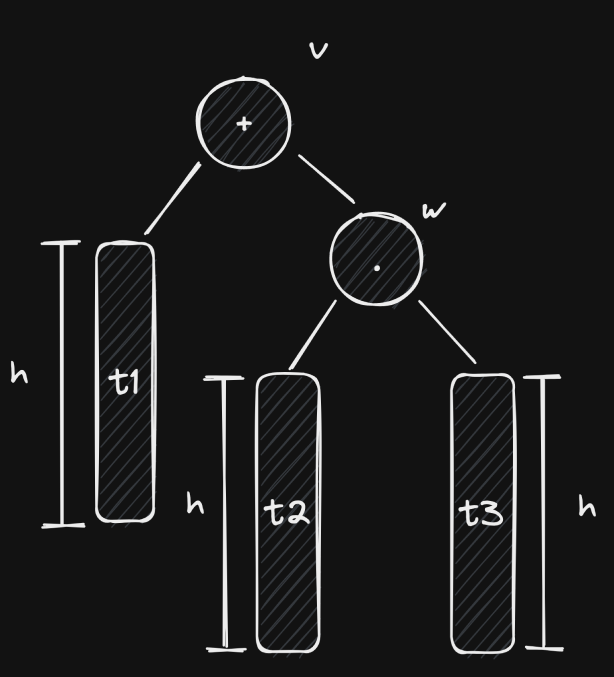
Case 1.1: $n$ is in $w$’s right subtree

If $n$ is in $t_3$, then $H(t_3) = h + 1$ and $BF(w) = 1$ after the insertion.

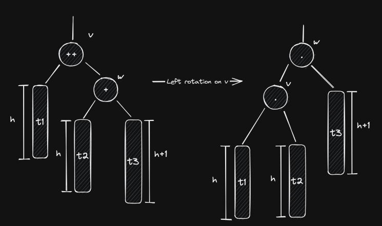
To get out of this scenario, we’re going to perform a left rotation on $v$. After it, $v$ becomes $w$’s left child and $t_2$ becomes $v$’s right child. Since $H(t_1) = H(t_2) = h$, this means that $BF(v) = 0$. This also means that now $H(v) = h+1$ and that $BF(w) = 0$. Everything’s balanced!

Case 1.2: $n$ is in $w$’s left subtree

If this is the case, then $w$ has a left child $x$ and our tree now looks like this:

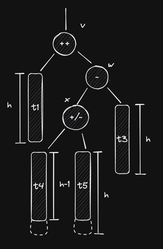
It is possible that $n = x$, in which case $h = 0$, but that’s not mandatory. We also can’t infer the exact height of $x$’s subtrees, but we know that at least one of them has height equal to $h$ (because $H(x) = h + 1$, so that $H(w) = 2$), leaving the other with value $h - 1$. $t_4$ and $t_5$ cannot end up with equal heights because we’re dealing with an insertion, and if $BF(w)$ changed after inserting, then so did $H(x)$, and that wouldn’t be happen if $H(t_4) = H(t_5)$. This means that either $BF(x) = 1$ or $BF(x) = -1$. Our solution will work regardless of these details.

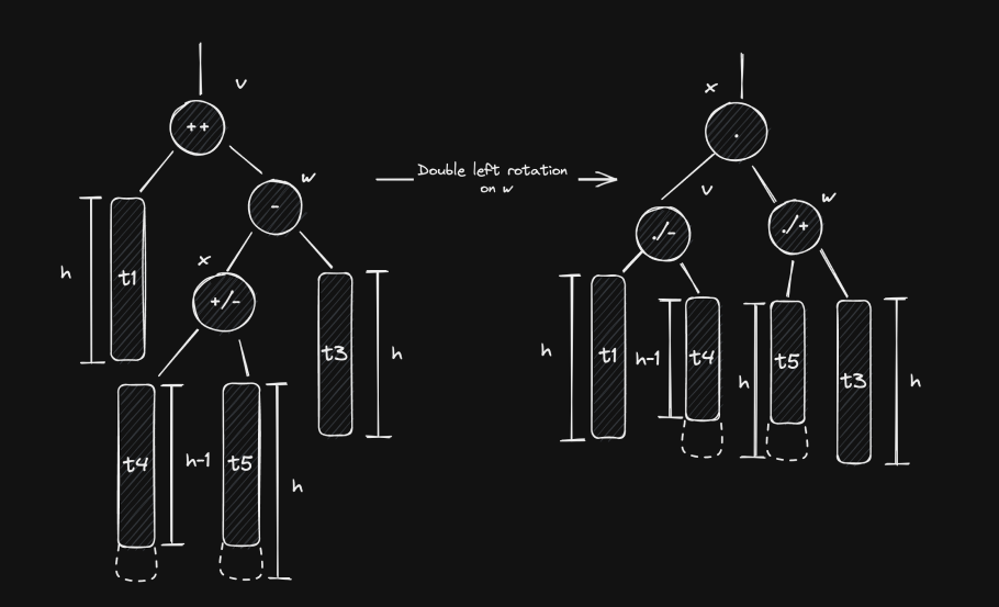
Notice how just a simple left (or right) rotation on $v$ isn’t the solution. As a matter of fact, it will make things worse (go ahead and check it)! This is because $n$ is in $w$’s left subtree, but $v$ is right-heavy. To solve this, we need to perform two rotations: a right rotation on $w$ followed by a left rotation on $v$. This is also called a right-left rotation or a double left rotation on $w$.

The final values for $BF(v)$ and $BF(w)$ both depend on the initial value of $BF(x)$ (prior to the insertion). This means that we can create two more sub-cases:

• Case 1.2.1: $BF(x) = 1$: if so, then $H(t_4) = h - 1$ and $H(t_5) = h$, implying that $BF(v) = -1$ and $BF(w) = 0$.
• Case 1.2.2: $BF(x) = -1$: then $H(t_4) = h$ and $H(t_5) = h - 1$, and therefore $BF(v) = 0$ and $BF(w) = 1$.

In both cases, $x$’s final balance factor is equal to 0 and the tree is balanced again.

Case 2: Removal in $v$’s left subtree

We return to our initial starting point, introduced before case 1. Except this time, $v$’s going to become unbalanced after a removal on $t_1$. Thus, $BF(v) = 2$ because $H(t_1) = h - 1$ and $H(w) = h+ 1$.

Even though we’re dealing with a removal, the possible sub-cases follow mostly the same structure as those from case 1. This is because the difference in height remains the same, it only happened due to a decrease of $v$’s left subtree, not an increase of its right. You’ll see that our strategies remain pretty much the same, with the exception of some final balance factor values:

• Case 2.1: $BF(w) \geq 0$: a left rotation on $v$ is used. Notice how it’s now possible for $BF(w) = 0$, since the changed subtree was $t_1$. This leads to some sub-cases with different final balance factors:
  • Case 2.1.1: $BF(w) = 1$: identical to case 1.1.
  • Case 2.1.2: $BF(w) = 0$: since $H(t_1) = h -1$ and $H(t_4) = h$, then $BF(v) = 1$. Similarly, due to $H(t_5) = h$ and $H(v) = h + 1$, then $BF(w) = -1$.
• Case 2.2: $BF(w) = -1$: a right-left rotation on $v$ is used, just like case 1.2. This case also has other sub-cases, which are determined by the possible values of $BF(x)$:
  • Case 2.2.1: $BF(x) = 1$: identical to case 1.2.1.
  • Case 2.2.2: $BF(x) = -1$: identical to case 1.2.2.
  • Case 2.2.3: $BF(x) = 0$: this new case is only possible with deletion. Here, we have that $H(t_4) = H(t_5) = h$, and thus $BF(v) = BF(w) = 0$.

The cases for when $BF(v) = -2$ (insertion in left subtree or removal from right) are simply mirrored versions of all these previous cases. I encourage you to try to work them out by yourself, it’ll deepen your understanding.

Implementation

Now we can start dealing with details. Overall, as I’ve already said, the main difference between implementing an AVL tree and a binary search tree is that we need to check if three has become unbalanced after an insert/removal and act accordingly. But this raises some questions.

First, how do we detect if the tree has become unbalanced? The most efficient way to do this is to just keep track of each node’s balance factor. At the end of the day, this just means one more field in your node object. Still, this adds the overhead of having to correctly update balance factors after insertions/removals.

This in turn leads to the question: after such an operation, which nodes’ balance factor should we update? Certainly, the father of a node that was just inserted/removed needs to have its balance factor updated, but does this propagate to the grandfather? What about the great-grandfather and beyond? Since every node’s balance factor is defined on terms of its children’s heights, then, generally speaking, for every node $v$ with parent $u$, a change in $BF(v)$ leads to a change in $BF(u)$ if, and only if, that change also alters $v$’s height.

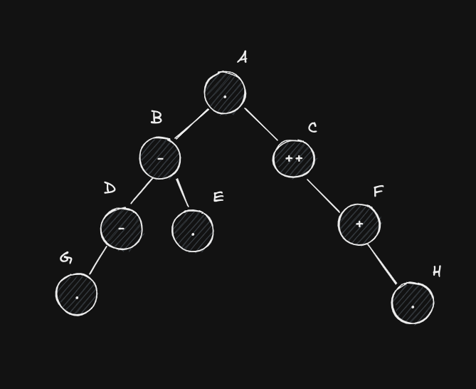
For example, consider the tree below. If we insert a node $E$ on $C$’s left subtree, that will change $C$’s balance factor (the father), but that doesn’t propagate to $A$ (the grandfather) because $C$’s height remains the same. On the other hand, if $D$ is deleted, that does propagate to $A$ because $C$’s height changes.

Now, how do we detect if an operation that changed $BF(v)$ also changed $H(v)$? We can use $BF(v)$ to determine which of $v$’s subtrees is the tallest. Since the height of any tree is simply the height of its tallest subtree plus one, then we can use $BF(v)$’s values before and after the operation to check if $v$’s tallest subtree (and thus $v$) has gotten taller or shorter. For example, if $BF(v) = 1$, then this means that $v_r$ is the tallest subtree. If, after an insertion, $BF(v)$ becomes 2, then this means that $v_r$ got taller and thus so did $v$. This also works when $BF(v) = 0$, since either one of the subtrees can be considered the tallest. On the other hand, if $BF(v)$ was -1 and it increased to 0 due to an insertion, then $v_l$ was the tallest but it didn’t increase in height and so neither did $v$.

There are also other cases for left-insertion and for the removal of nodes. Here’s a quick summary:

• If the operation was an insertion, then $H(v)$ only increases if:
  • $v_r$ was its tallest subtree ($BF(v) \geq 0$) and $BF(v)$ increases after the insertion.
  • $v_l$ was its tallest subtree ($BF(v) \leq 0$) and $BF(v)$ decreases after the insertion.
• If the operation was a removal, then $H(v)$ only decreases if:
  • $BF(v)$ was equal to 1 and then becomes 0 after the removal.
  • $BF(v)$ was equal to -1 and then it becomes 0 after the removal.

Can you guess why, if $BF(v) = 0$ prior to a removal, a subsequent decrease/increase in $BF(v)$ doesn’t cause $H(v)$ to change?

Lastly, what nodes do we check after an operation? We have to check every node on the path from the tree’s root to the place where the operation took place, as all of these nodes are subject to unbalance.

With all of this in mind, here’s a JavaScript implementation of an AVL tree with insert and delete methods. An important thing to notice here is how we need to determine, when rotating, in what specific case we’re in (insertion or removal and their sub-cases) so that the balance factors can be updated accordingly.

class AVLNode {
  constructor(value) {
    this.value = value;
    this.bf = 0; // balance factor
    this.left = null;
    this.right = null;
  }
}

class AVLTree {
  #root = null;

  // Client-facing method with a friendlier signature.
  add(value) {
    this.#root = this.#insert(this.#root, null, value);
  }

  // Actual recursive insert method, follows the same overall structure as
  // a regular binary search tree insert.
  #insert(node, parent, value) {
    if (node === null) {
      node = new AVLNode(value);
      // We always update the balance factor of the father after
      // inserting/removing.
      if (parent !== null) {
        if (value > parent.value) parent.bf += 1;
        else parent.bf -= 1;
      }
      return node;
    }

    let prevBf = node.bf;
    if (value > node.value) {
      node.right = this.#insert(node.right, node, value);
      // The change in the balance factor only propagates to the father
      // if the node's tallest subtree increased.
      if (parent !== null && prevBf >= 0 && node.bf > prevBf) {
        if (node.value > parent.value) parent.bf += 1;
        else parent.bf -= 1;
      }

      if (node.bf === 2) {
        // The node is unbalanced. Need to determine what case we're in
        // so that we can choose the appropriate strategy.
        let w = node.right;
        // Case 1.1
        if (value > w.value) node = this.#rotateLeft(node, parent);
        // Case 1.2
        else node = this.#rotateRightLeft(node, parent);
      }
    } else if (value < node.value) {
      // These are simply mirror cases of the right-insert ones.
      node.left = this.#insert(node.left, node, value);
      if (parent !== null && prevBf <= 0 && node.bf < prevBf) {
        if (node.value > parent.value) parent.bf += 1;
        else parent.bf -= 1;
      }
      if (node.bf === -2) {
        let w = node.left;
        if (value < w.value) node = this.#rotateRight(node, parent);
        else node = this.#rotateLeftRight(node, parent);
      }
    }
    return node;
  }

  delete(value) {
    this.#root = this.#remove(this.#root, null, value);
  }

  #remove(node, parent, value) {
    if (node === null) return null;
    let prevBf = node.bf;
    if (value > node.value) {
      node.right = this.#remove(node.right, node, value);
      if (parent !== null && prevBf === 1 && node.bf === 0) {
        if (node.value > parent.value) parent.bf -= 1;
        else parent.bf += 1;
      }
      if (node.bf === -2) {
        let w = node.left;
        if (w.bf <= 0) node = this.#rotateRight(node, parent);
        else node = this.#rotateLeftRight(node, left);
      }
    } else if (value < node.value) {
      node.left = this.#remove(node.left, node, value);
      // We only propagate the change if the tallest subtree
      // has become shorter.
      if (parent !== null && prevBf === -1 && node.bf === 0) {
        if (node.value > parent.value) parent.bf -= 1;
        else parent.bf += 1;
      }

      // Notice how these if blocks mirror those of the insertion method
      // for when node.bf === 2.
      if (node.bf === 2) {
        let w = node.right;
        // Case 2.1
        if (w.bf >= 0) node = this.#rotateLeft(node, parent);
        // Case 2.2
        else node = this.#rotateRightLeft(node, parent);
      }
    } else {
      // We always update the balance factor of the father after
      // inserting/removing.
      if (parent !== null && node.value > parent.value) parent.bf -= 1;
      else if (parent !== null) parent.bf += 1;

      if (node.left === null) return node.right;
      if (node.right === null) return node.left;

      const succ = this.#successor(node);
      succ.right = this.#remove(node.right, node, succ.value);
      succ.left = node.left;
      // Notice how, since the successor essentially takes the place of
      // the removed node, it also inherits its balance factor
      // after the removal of the successor from the right subtree.
      succ.bf = node.bf;
      return succ;
    }
    return node;
  }

  #successor(node) {
    let current = node.right;
    while (current.left !== null) {
      current = current.left;
    }
    return current;
  }

  // Possible cases for rotating left: 1.1, 2.1.1 and 2.1.2
  #rotateLeft(v, parent) {
    const w = v.right;
    const t2 = w.left;
    w.left = v;
    v.right = t2;
    if (parent !== null) {
      if (v.value > parent.value) parent.right = w;
      else parent.left = w;
    }

    // Case 2.1.2
    if (w.bf === 0) {
      w.bf = -1;
      v.bf = 1;
    } else {
      // Cases 1.1 and 2.1.1
      v.bf = 0;
      w.bf = 0;
    }

    return w;
  }

  // Possible cases for rotating right-left: 1.2.1, 1.2.2, 2.2.1, 2.2.2 and 2.2.3
  #rotateRightLeft(v, parent) {
    const w = v.right;
    // Rotating w right
    const x = w.left;
    w.left = x.right;
    x.right = w;
    v.right = x;
    // Rotating v left
    v.right = x.left;
    x.left = v;
    if (parent !== null) {
      if (v.value > parent.value) parent.right = x;
      else parent.left = x;
    }

    // Case 2.2.3
    if (x.bf === 0) {
      v.bf = 0;
      w.bf = 0;
    } else if (x.bf === 1) {
      // Cases 1.2.1 and 2.2.1
      v.bf = -1;
      w.bf = 0;
    } else {
      // Cases 1.2.2 and 2.2.2
      v.bf = 0;
      w.bf = 1;
    }
    x.bf = 0;
    return x;
  }

  #rotateRight(v, parent) {
    const w = v.left;
    const t2 = w.right;
    w.right = v;
    v.left = t2;
    if (parent !== null) {
      if (v.value > parent.value) parent.right = w;
      else parent.left = w;
    }

    if (w.bf === 0) {
      w.bf = 1;
      v.bf = -1;
    } else {
      v.bf = 0;
      w.bf = 0;
    }

    return w;
  }

  #rotateLeftRight(v, parent) {
    const w = v.left;
    const x = w.right;
    x.left = w;
    w.right = x.left;
    v.left = x;
    v.left = x.right;
    x.right = v;
    if (parent !== null) {
      if (v.value > parent.value) parent.right = x;
      else parent.left = x;
    }

    if (x.bf === 0) {
      v.bf = 0;
      w.bf = 0;
    } else if (x.bf === 1) {
      v.bf = 0;
      w.bf = -1;
    } else {
      v.bf = 1;
      w.bf = 0;
    }
    x.bf = 0;
    return x;
  }

Conclusion

That’s it, we’re done!

This article contained quite a bit of theory, so make sure to re-read it, as it can be very tough (I’d say impossible, at least for me) to really absorb all of these details in just one read, especially if you’ve never encountered AVL trees before.

I was aiming to be as detailed as possible when writing this, as the resources I used for studying this topic were a bit “dry”, which forced me to piece a lot of things by myself. Nevertheless, this did give me a better understanding on these structures and why they work the way they do, so I tried to find a balance between these two approaches.

The next article in this series will probably be about B-trees and how they’re used in all sorts of places, like database indices and file-systems. Stay tuned for that! See ya!